Archive
Self Service BI by using Power BI – Power Pivot (Part 2)
After a long pause I’m back again to discuss on Power BI.
In my previous Power BI Series first part [link] I discussed about the first component of Power BI, i.e. Power Query and how to use it to discover and gather data.
Power Pivot lets you:
1. Create your own Data Model from various Data Sources, Modeled and Structured to fit your business needs.
2. Refresh from its Original sources as often as you want.
3. Format and filter your Data, create Calculated fields, define Key Performance Indicators (KPIs) to use in PivotTables and create User-Defined hierarchies to use throughout a workbook.
And here in second part I will discuss about few of these features.
–> The benefit of creating Data Model in Power Pivot is that Power Pivot Models run in-memory so that users can analyze 100’s of millions of rows of data with lightning fast performance.
All you need is Microsoft Excel 2013 to create your Data Model. Check this [link] to troubleshoot if you don’t see POWERPIVOT option in Excel ribbon.
–> Creating Data Model:
To create a Data Model you need a Data Source, so we will use SQL Server as a Data Source and I’ve setup AdventureWorksDW2012 Database for our hands-on. Click [here] to download AdventureWorksDW2012 DB from CodePlex.
1. Open Excel, and go to POWERPIVOT tab and click on Manage, this will open a new PowerPivot Manager window.

2. Now on this new window, click on From Database icon and select From SQL Server from the dropdown, this will open a Table Import Wizard Popup window.
3. Provide SQL Server Instance name that you want to connect to. Select AdventureWorksDW2012 Database from the Database name dropdown, and click Next.

4. Click Next again and select the required Tables (10 selected), click Finish.

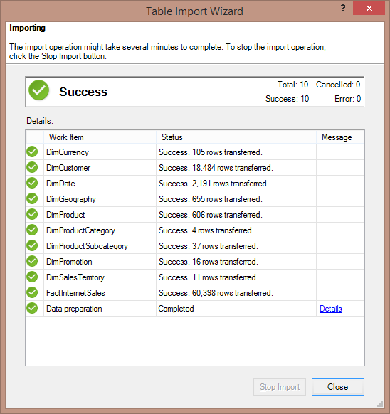
5. Make sure you get Success message finally, click Close.
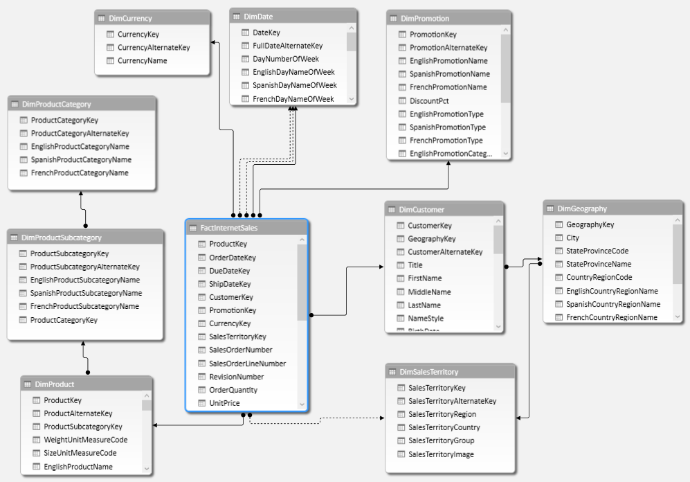
6. In the PowerPivot Manager window you will see many tabs listing records. Click on Diagram View to see all the tabs as tables and relations between them. This is your Power Pivot – Data Model:
–> Now as your Data Model is ready, you can create Pivot Reports in Excel, let’s see how:
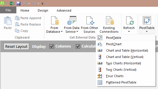
1. Go to the PowerPivot Manager window and click on PivotTable icon and then select PivotTable from the dropdown.
2. The control moves to the Excel sheet, select Existing Worksheet on the Popup.
3. Now select following columns form the PivotTable Fields list:
– DimGeography.EnglighCountryRegionName
– FactInternetSales.SalesAmount
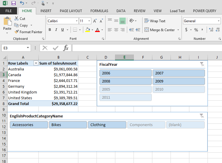
This would give you Total sales across Regions in the Worksheet
4. Let’s add some Slicers to this:
4.a. Click on PIVOTTABLE TOOLS – ANALYZE, here click on Insert Slicer. On ALL tab, select DimDate.FiscalYear column. This will add Year slicer to the report.
4.b. Now again click on the PivotTable Report, you will see the PIVOTTABLE TOOLS on the ribbon bar again. Select Insert Slicer again and select DimProductCategory.EnglighProductCategoryName column.
You can align, move, resize the report, slicers and beautify the report as you want, as shown below:
This way you can add Graphs, Charts and create very impressive Reports UI as per your requirements.
This Power Pivot – Data Model can also be used to create Power View Reports, which we will cover in next part of this series.
Thanks!!!


![]()
Current Visitors

StatCounter …since April 2012

 Leisure blog: Creek & Trails
- NMDC Hyderabad Marathon – My first 42k FM, cramps, training and fuelling
- Singapore (Part 2) – 6 days itinerary, sightseeing & attractions
- Singapore (Part 1) – Tickets, Visa, Hotel, Forex Card/Cash, Metro/Bus cards
- I got full refund of my flight tickets during COVID lockdown (AirIndia via MakeMyTrip)
- YouTube – Your Google Ads account was cancelled due to no spend
- YouTube latest update on its YPP (YouTube Partner Program) which may affect your channel
- Starting your own blog !!!
- How to file ITR (Income Tax Return) online AY 2017-18 (for simple salaried)
- Scam – Become a kin/hier and earn a fortune – via LinkedIn and Email
- Places to visit in and around Vizag (aka Visakhapatnam)
