Differences | SQL with Manoj

SQL Server CROSS APPLY and OUTER APPLY usage – MSDN TSQL forum

May 29, 2016 Leave a comment

–> Question:

I need to see two small scenario when people should use CROSS APPLY and OUTER APPLY.

Please discuss the scenario with code and example.

Thanks !

–> My Answer:

CROSS APPLY acts like an INNER JOIN, and OUTER APPLY acts like a LEFT OUTER JOIN.

–> The APPLY clause (irrespective of CROSS/OUTER option) gives you flexibility to pass table’s columns as parameters to UDFs/functions while Joining while that table. It was not possible with JOINS. The function will execute for each row value passed to the UDF as parameter. But the JOIN works as a whole set.

Check the blog post on CROSS APPLY vs OUTER APPLY operators, https://sqlwithmanoj.com/2010/12/11/cross-apply-outer-apply/

–> Apart from this you can also use APPLY clause with Tables/SubQueries, like if you want to get top 5 products sold by sales persons, or get top 10 populated Cities from all States.

Check here: Using CROSS APPLY & OUTER APPLY operators with UDFs, Derived-Tables/Sub-Queries & XML data, https://sqlwithmanoj.com/2012/01/03/using-cross-apply-outer-apply-operators-with-udfs-derived-tables-xml-data/

–> Answer from Russ Loski:

First let’s start with the use for APPLY.

You would use APPLY if you need to use a column from a table as an argument in a derived table or function. For example, this query from http://blog.sqlauthority.com/2009/08/21/sql-server-get-query-plan-along-with-query-text-and-execution-count/:

SELECT cp.objtype AS ObjectType,
OBJECT_NAME(st.objectid,st.dbid) AS ObjectName,
cp.usecounts AS ExecutionCount,
st.TEXT AS QueryText,
qp.query_plan AS QueryPlan
FROM sys.dm_exec_cached_plans AS cp
CROSS APPLY sys.dm_exec_query_plan(cp.plan_handle) AS qp
CROSS APPLY sys.dm_exec_sql_text(cp.plan_handle) AS st
--WHERE OBJECT_NAME(st.objectid,st.dbid) = 'YourObjectName'

I need to use columns from dm_exec_cahced_plans to pass to two functions to get rows from those functions. I have to use the APPLY keyword (rather than Join) to be able to do that.

I can do the same with a derived table:

SELECT * 
FROM TableA 
outer apply (
SELECT * from TableB
where TableA.id = TableB.id
) tb2

That is a horrible example (you can do the same using standard join syntax). But there are very rare circumstances where I need to use a column in a where clause in a derived table, but I can’t use a join.

The difference between CROSS APPLY and OUTER APPLY is the difference between INNER JOIN and OUTER JOIN. CROSS APPLY will only return rows where there is a row in both the first table and the second table/function, while OUTER APPLY returns a row if there is a row in the first Table even if the second table/function returns no rows.

Ref link.

Categories: Differences Tags: APPLY Operator, CROSS APPLY, MSDN TSQL forum, OUTER APPLY

SQL Trivia – Difference between COUNT(*) and COUNT(1)

January 13, 2016 3 comments

Yesterday I was having a discussion with one of the Analyst regarding an item we were going to ship in the release. And we tried to check and validate the data if it was getting populated correctly or not. To just get the count-diff of records in pre & post release I used this Query:

SELECT COUNT(*) FROM tblXYZ

To my surprise he mentioned to use COUNT(1) instead of COUNT(*), and the reason he cited was that it runs faster as it uses one column and COUNT(*) uses all columns. It was like a weird feeling, what to say… and I just mentioned “It’s not, and both are same”. He was adamant and disagreed with me. So I just kept quite and keep on using COUNT(*) 🙂

But are they really same or different? Functionally? Performance wise? or by any other means?

Let’s check both of them.

The MSDN BoL lists the syntax as COUNT ( { [ [ ALL | DISTINCT ] expression ] | * } )

So, if you specify any numeric value it come under the expression option above.

Let’s try to pass the value as 1/0, if SQL engine uses this value it would definitely throw a “divide by zero” error:

SELECT COUNT(1/0) FROM [Person].[Person]

… but it does not. Because it just ignores the value while taking counts. So, both * and 1 or any other number is same.

–> Ok, let’s check the Query plans:

and there was no difference between the Query plans created by them, both have same query cost of 50%.

–> These are very simple and small queries so the above plan might be trivial and thus may have come out same or similar.

So, let’s check more, like the PROFILE stats:

SET STATISTICS PROFILE ON
SET STATISTICS IO ON

SELECT COUNT(*) FROM [Sales].[SalesOrderDetail]

SELECT COUNT(1) FROM [Sales].[SalesOrderDetail]

SET STATISTICS PROFILE OFF
SET STATISTICS IO OFF

If you check the results below, the PROFILE data of both the queries shows COUNT(*), so the SQL engine converts COUNT(1) to COUNT(*) internally.

SELECT COUNT(*) FROM [Sales].[SalesOrderDetail]
  |--Compute Scalar(DEFINE:([Expr1002]=CONVERT_IMPLICIT(int,[Expr1003],0)))
       |--Stream Aggregate(DEFINE:([Expr1003]=Count(*)))
            |--Index Scan(OBJECT:([AdventureWorks2014].[Sales].[SalesOrderDetail].[IX_SalesOrderDetail_ProductID]))

SELECT COUNT(1) FROM [Sales].[SalesOrderDetail]
  |--Compute Scalar(DEFINE:([Expr1002]=CONVERT_IMPLICIT(int,[Expr1003],0)))
       |--Stream Aggregate(DEFINE:([Expr1003]=Count(*)))
            |--Index Scan(OBJECT:([AdventureWorks2014].[Sales].[SalesOrderDetail].[IX_SalesOrderDetail_ProductID]))

–> On checking the I/O stats there is no difference between them:

Table 'SalesOrderDetail'. Scan count 1, logical reads 276, physical reads 1, 
 read-ahead reads 288, lob logical reads 0, lob physical reads 0, lob read-ahead reads 0.

Table 'SalesOrderDetail'. Scan count 1, logical reads 276, physical reads 0, 
 read-ahead reads 0, lob logical reads 0, lob physical reads 0, lob read-ahead reads 0.

Both the queries does reads of 276 pages, no matter they did logical/physical/read-ahead reads here. Check difference b/w logical/physical/read-ahead reads.

So, we can clearly and without any doubt say that both COUNT(*) & COUNT(1) are same and equivalent.

There are few other things in SQL Server that are functionally equivalent, like DECIMAL & NUMERIC datatypes, check here: Difference b/w DECIMAL & NUMERIC datatypes.

Categories: Differences, Misconception Tags: SQL Count

Difference between Index and Primary Key – MSDN TSQL forum

August 10, 2015 Leave a comment

–> Question:

What is the difference between the Index and the Primary Key?

–> My Answer:

In simple DBMS words:

– A Primary Key is a constraint or a Rule that makes sure to identify a table’s column uniquely and enforces it contains a value, ie. NOT NULL value.

– An Index on the other side is not a constraint, but helps you organize the table or selected columns to retrieve rows faster while querying with SELECT statement.

In SQL Server you can create only one Primary Key, and by-default it creates a Clustered Index on the table with the PK column as the Index key. But you can specify to create Non-Clustered Index with a PK also.

Indexes in SQL Server mainly are:

– Clustered Index

– Non Clustered

… you can specify them as unique or non-unique.

Other type of indexes are:

– ColumnStore

– Filtered

– XML

– Spatial

– Full Text

–> Another Answer by Erland:

A primary key is a logical concept. The primary key are the column(s) that serves to identify the rows.

An index is a physical concept and serves as a means to locate rows faster, but is not intended to define rules for the table. (But this is not true in practice, since some rules can only be defined through indexes, for instance filtered indexes.)

In SQL Server a primary key for a disk-based table is always implemented as an index. In a so-called memory-optimized table, the primary key can be implemnted as an index or as a hash.

–> Another Answer by CELKO:

PRIMARY KEY is define in the first chapter of the book on RDBMS you are too lazy to read. It is a subset of columns in the table which are all not null and unique in the table. An index is an access method used on the records of a physical file.

Many SQL products use indexes to implement keys; many do not (hashing is a better way for large DB products)

Check the video on Primary Keys:

Ref link.

Categories: Differences, SQL Server Questions Tags: Index, MSDN TSQL forum, PRIMARY KEY

SQL Basics – Difference between WHERE, GROUP BY and HAVING clause

May 23, 2015 6 comments

All these three Clauses are a part/extensions of a SQL Query, are used to Filter, Group & re-Filter rows returned by a Query respectively, and are optional. Being Optional they play very crucial role while Querying a database.

–> Here is the logical sequence of execution of these clauses:

1. WHERE clause specifies search conditions for the rows returned by the Query and limits rows to a meaningful set.

2. GROUP BY clause works on the rows returned by the previous step #1. This clause summaries identical rows into a single/distinct group and returns a single row with the summary for each group, by using appropriate Aggregate function in the SELECT list, like COUNT(), SUM(), MIN(), MAX(), AVG(), etc.

3. HAVING clause works as a Filter on top of the Grouped rows returned by the previous step #2. This clause cannot be replaced by a WHERE clause and vice-versa.

As these clauses are optional thus a minimal SQL Query looks like this:

SELECT *
FROM [Sales].[SalesOrderHeader]

This Query returns around 32k (thousand) rows form SalesOrderHeader table. Thus, if somebody wants to do some analysis on this big row-set it would be very difficult and time consuming for him.

–> Use Case: Let’s say a Sales department wants to get a list of such Customers who bought more number of items last year, so that they can sell more some stuff to them this year. How they will go ahead?

1. Using WHERE clause: First of all they will need to apply filter on above ~32k rows and get list of Orders that were made last year (i.e. in 2014) to limit the row-set, like:

SELECT *
FROM [Sales].[SalesOrderHeader]
WHERE OrderDate >= '2014-01-01 00:00:00.000'
AND OrderDate < '2015-01-01 00:00:00.000'

This Query still gives ~12k records and its still difficult to identify such Customers who have more orders.

2. Using GROUP BY clause: Here we need to group the Customers with their number of Orders, like:

SELECT CustomerID, COUNT(*) AS OrderNos
FROM [Sales].[SalesOrderHeader]
WHERE OrderDate >= '2014-01-01 00:00:00.000'
AND OrderDate < '2015-01-01 00:00:00.000'
GROUP BY CustomerID

This query still returns ~10k records, and I’ve go through the entire list of records to identify such records. Is there any way where I can still filter out the unwanted records with lesser count?

3. USING HAVING clause: This will works on top of GROUP BY clause to filter the grouped records onCOUNT(*) AS OrderNos column values (like a WHERE clause), like:

SELECT CustomerID, COUNT(*) AS OrderNos
FROM [Sales].[SalesOrderHeader]
WHERE OrderDate >= '2014-01-01 00:00:00.000'
AND OrderDate < '2015-01-01 00:00:00.000'
GROUP BY CustomerID
HAVING COUNT(*) > 10

Thus, by using all these these clauses we can reduce and narrow down the row-set to do some quick analysis.

Check this video tutorial on WHERE clause and difference with GROUP BY & HAVING clause.

Categories: Differences, SQL Basics Tags: GROUP BY, GROUP BY vs HAVING, HAVING, WHERE

What is SQL, PL/SQL, T-SQL and difference between them

May 3, 2015 16 comments

Today I got an email from a student who is pursuing his Bachelors degree in Computer Application (BCA). He visited my blog and sent me an email regarding his confusion with terms like SQL, T-SQL, PL/SQL, and asked me what is differences between them and how are they related? I had a chat with him and told the basic differences, but he further asked me how they are related to Microsoft SQL Server, Oracle, MySQL, etc? As he is studying SQL only based upon Oracle in his course curriculum, these all terms were not clear to him, so I cleared all his doubts while chatting with him.

After a while I had a same reminiscence that when I was a student I also had these doubts and confusions, and there was nobody to guide me, but I gradually came to know about this and it took some time. Thus, I’am taking this opportunity to put all these things together here in a single blog post for my readers (specially students) and for my reference as well.

–> SQL: stands for Structured Query Language and is pronounced as Sequel, and in early days it was also known as SEQUEL only.

– IBM in early 1970s developed SEQUEL which stands for Structured English QUEry Langauge for their RDBMS. The acronym was later changed to SQL, as SEQUEL was already trademarked by some UK based aircraft company.

–> PL/SQL: stands for Procedural Language/Structured Query Language and is used with Oracle database to create PL/SQL units such as Procedures, Functions, Packages, Types, Triggers, etc. which are stored in the database for reuse by applications that use any of the Oracle Database programmatic interfaces.

– Oracle in 1970s known as “Relational Software” saw SQL potential and influenced by Boyce, Codd and Chamberlin developed their own RDBMS product which was commercially available as Oracle Database. Oracle is supported on many Operating Systems like Windows, Linux, Solaris, AIX, OpenVMS, etc. [Oracle Database]

–> DB2: IBM during early 1980s made SQL commercially available with its product known as IBM DB2 from its prototype “System R”. [IBM DB2]

–> SQL Standardization: Later in 1986 SQL was adopted as a Standard by ANSI (American National Standards Institute) as SQL-86, and today the latest Standard is known as SQL:2011

✔ As a standarg SQL should support following:

– Language elements: Clauses, Expressions, Predicates, Queries, Statements.
– Operators: =, , >, =, <=, BETWEEN, LIKE, IN, NOT IN, IS, IS NOT, AS, etc.
– Conditional expressions: CASE, IF ELSE
– Queries: which include SELECT, FROM, WHERE, GROUP BY, HAVING, ORDER BY, etc.
– Data Types: Numeric, Char, Bit, Date and Time
– NULL or 3VL (Three value Logic)
– DDL, DML, TCL

–> T-SQL: stands for Transact-SQL, and is Sybase & Microsoft’s proprietary extension. T-SQL is very similar to PL/SQL, one can create T-SQL units such as Procedures, Functions, Types, Triggers, etc. as mentioned above.

– In 1987 Sybase shipped their first RDBMS product known as Sybase SQL Server. [Sybase]

– In 1988-89 Microsoft had an agreement with Sybase and ported the Sybase RDBMS to OS/2 platform and marketed it as Microsoft SQL Server 1.0, which was equivalent to Sybase SQL Server 3.0. [Microsoft SQL Server]

– In 1993 Sybase and Microsoft dissolved their partnership, and Microsoft bought the SQL Server code base from Sybase and both went different streams to develop their own product.

– Till SQL Server 2000 Microsoft has Sybase code base, and this was completely written in SQL Server 2005.

– Microsoft SQL Server is only supported on Windows Operating Systems.

–> MySQL: was founded by a Swedish Company MySQL AB in 1995 and is the most widely used open-source RDBMS. The MySQL development project has made its source code available under the terms of the GNU General Public License. MySQL does not currently comply with the full SQL standard. In 2008 Oracle corporation completely acquired MySQL. MySQL is supported on many Operating Systems like Windows, Linux, Solaris, OS X and FreeBSD. [MySQL.com]

–> FoxPRO and dBase: were very popular DataBase Management System (DBMS) products in mid 1980s and 1990s. They lack some RDBMS features and are out of support now, but are still being used in various legacy systems.

– FoxPRO is supported by Microsoft and was a text-based Procedural programming language and DBMS, for MD DOS, Windows, and UNIX. Microsoft Visual FoxPRO 9.0 being the latest and probably the last version published in 2007. [FoxPRO msdn]

– dBase was a very popular DBMS package including core Database engine, a Query system, a Forms engine and a xBase programming language with *.dbf file format. [dBase.com]

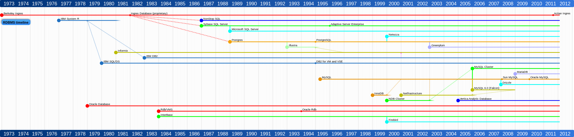
–> Here is a complete timeline that shows SQL and how it got evolved as different Products by different Vendors/Companies (click on the image to expand):

–> There are many other popular SQL Products/System softwares available in market, and major of them are:
1. Oracle database
2. Microsoft SQL Server
3. IBM DB2
4. MySQL
5. PostgreSQL
6. Teradata

Create a software development environment with a tool such as Visual Studio and access it from any where on any device on your hosted virtual desktop from CloudDesktopOnline.com. Also, if you prefer a server, try Apps4Rent.