Archive
Self Service BI by using Power BI – Power Pivot (Part 2)
After a long pause I’m back again to discuss on Power BI.
In my previous Power BI Series first part [link] I discussed about the first component of Power BI, i.e. Power Query and how to use it to discover and gather data.
Power Pivot lets you:
1. Create your own Data Model from various Data Sources, Modeled and Structured to fit your business needs.
2. Refresh from its Original sources as often as you want.
3. Format and filter your Data, create Calculated fields, define Key Performance Indicators (KPIs) to use in PivotTables and create User-Defined hierarchies to use throughout a workbook.
And here in second part I will discuss about few of these features.
–> The benefit of creating Data Model in Power Pivot is that Power Pivot Models run in-memory so that users can analyze 100’s of millions of rows of data with lightning fast performance.
All you need is Microsoft Excel 2013 to create your Data Model. Check this [link] to troubleshoot if you don’t see POWERPIVOT option in Excel ribbon.
–> Creating Data Model:
To create a Data Model you need a Data Source, so we will use SQL Server as a Data Source and I’ve setup AdventureWorksDW2012 Database for our hands-on. Click [here] to download AdventureWorksDW2012 DB from CodePlex.
1. Open Excel, and go to POWERPIVOT tab and click on Manage, this will open a new PowerPivot Manager window.

2. Now on this new window, click on From Database icon and select From SQL Server from the dropdown, this will open a Table Import Wizard Popup window.
3. Provide SQL Server Instance name that you want to connect to. Select AdventureWorksDW2012 Database from the Database name dropdown, and click Next.

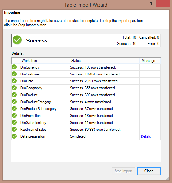
4. Click Next again and select the required Tables (10 selected), click Finish.

5. Make sure you get Success message finally, click Close.
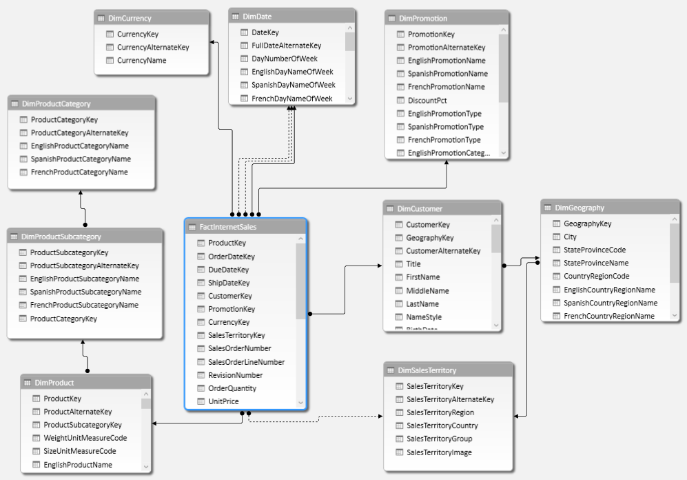
6. In the PowerPivot Manager window you will see many tabs listing records. Click on Diagram View to see all the tabs as tables and relations between them. This is your Power Pivot – Data Model:
–> Now as your Data Model is ready, you can create Pivot Reports in Excel, let’s see how:
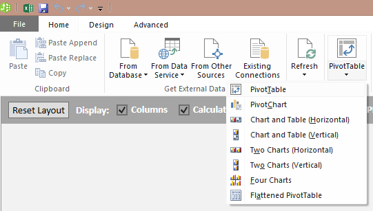
1. Go to the PowerPivot Manager window and click on PivotTable icon and then select PivotTable from the dropdown.
2. The control moves to the Excel sheet, select Existing Worksheet on the Popup.
3. Now select following columns form the PivotTable Fields list:
– DimGeography.EnglighCountryRegionName
– FactInternetSales.SalesAmount
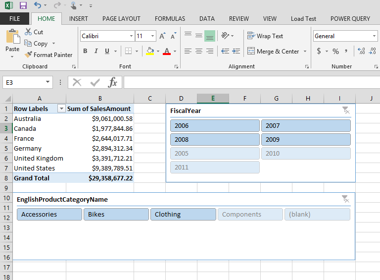
This would give you Total sales across Regions in the Worksheet
4. Let’s add some Slicers to this:
4.a. Click on PIVOTTABLE TOOLS – ANALYZE, here click on Insert Slicer. On ALL tab, select DimDate.FiscalYear column. This will add Year slicer to the report.
4.b. Now again click on the PivotTable Report, you will see the PIVOTTABLE TOOLS on the ribbon bar again. Select Insert Slicer again and select DimProductCategory.EnglighProductCategoryName column.
You can align, move, resize the report, slicers and beautify the report as you want, as shown below:
This way you can add Graphs, Charts and create very impressive Reports UI as per your requirements.
This Power Pivot – Data Model can also be used to create Power View Reports, which we will cover in next part of this series.
Thanks!!!
Import Excel Sheet with multiple Recordsets
Importing records from an Excel is a very simple task. Load your data in Excel with appropriate headers and Run the Import/Export Wizard, your records are transfered from Excel sheet to a MS SQL table.
But what if a single Sheet contains multiple record sets with variable headers. Like First 100 rows of Customer data with 10 headers. Then just below 50 rows of Order data with less than 10 or more than 10 headers.
Seems a bit difficult but not impossible. Its tricky though, lets see how:
Lets us suppose your Excel file is in following format shown in image below (Fig-1):
1. Contact recordset &
2. Sales Order recordset

Fig-1 Sheet with multiple recordsets
Now select the Contact recordset including headers as shown in Fig-2 and right-click and select “Name a Range…” option.

Fig-2 Create a named Range
Fig-3 shows a pop-up box where you can apply and provide a name for that range selection.

Fig-3 Range name for Contacts
Similarly repeat this for Sales Order recordset as shown in Fig-4.

Fig-4 Range name for Sales Order
Now you can see 2 named ranges Contacts & Sales in the dropdown in Fig-5.

Fig-5 Check both the Named ranges
Now we are ready to Import the data. As shown in Fig-6 the Import/Export wizard detects the named ranges and explicitly shows them as Source among other 3 sheets of your Excel file. Simply select both of them and make the required changes as you do for Sheets and click the Next button.

Fig-6 Named ranges while Import
Fig-7 Shows both the tables created & data loaded in SQL Server.

Fig-7 Sources getting copied into SQL tables
Now check the records and match them with the Excel sheet, as shown in Fig-8

Fig-8 Check the tables in SQL Server finally
Wow!!! that was simple.
I was asked this question in an SQL interview and I didn’t knew the answer, obviously you don’t need to know everything… but you should. Discussed this question on MSDN TSQL forum and got the suggestion, thus the blog post. Link: http://social.msdn.microsoft.com/Forums/en-US/transactsql/thread/cf849418-d18f-4b7a-99eb-dbfed6269603/#778c0e99-368a-40f2-b9d4-b747c1754853
Excel data validation with VBA macros
You have an important lead set or any other orders/financial recordset in excel and have to import the data in SQL Server. This is not a one time effort but ongoing and in future you have to deals with lot such records/data files. To import valid data in your SQL tables you want to ensure and validate at the frst step instead of correcting the data by firing SQL queries. Also to avoid this manual work to identify the incorrect/invalid data out of thousands of records automated approach would be quite helpful.
Excel not only store data but also have a power to run VBA macro code against and manipulate the data. Lets take a simple example to validate a set of Customer numbers & their insert date, shown below:
-- Test Data which is correct and expected to import in SQL table.
InsertDate	CustomerNo
11/16/2009	91878552
11/16/2009	101899768
11/16/2009	101768884
11/16/2009	123456789123
11/16/2009	101768800
Columns InsertDate should be a valid date & CustomerNo should be numeric & less than 12 characters or max length equal to 12.
-- Lets tweak the test data put some invalid values under both the columns, shown below:
InsertDate	CustomerNo
11/16/2009	91878552
51/96/2009	101899768
11/16/2009	1017abc84
11/16/2009	123456789123
11/16/2009	101768800
If you are on MS Office 2007 create a Macro enabled excel file with extension *.xlsm, OR if you are on 2003 and lower version *.xls file would be fine. Copy the above data in Sheet1 with incorrect values. Now press open up the VBA macro editor or press ALT+F11 keys. Now double click on Sheet1 under “Project -VBAProjects” explorer.
I wish to run the validation while someone tries to save the macro enabled excel file. So the event selected is “BeforeSave”. And the VBA macro code goes below:
Private Sub Workbook_BeforeSave(ByVal SaveAsUI As Boolean, Cancel As Boolean)

	Dim errorCode As Integer
	Dim errorMsg As String

	Dim numOfRecs As Integer
	Dim counter As Integer

	'---------------------
	'Start - Validate Date
	'---------------------
	Sheet1.Activate
	Range("A2").Select

	errorCode = 0
	numOfRecs = 0

	Do Until ActiveCell.Value = vbNullString

		' Validate Date
		If IsDate(ActiveCell.Value) <> True Then
			errorCode = 1
			ActiveCell.Interior.ColorIndex = 3 'Red
		Else
			ActiveCell.Interior.ColorIndex = 2 'White
		End If

		numOfRecs = numOfRecs + 1

		ActiveCell.Offset(1, 0).Select

	Loop

	If errorCode = 1 Then
		errorMsg = errorMsg + vbCrLf & "- Invalid Insert Date"
	End If
	'-------------------
	'End - Validate Date
	'-------------------

	'--------------------------
	'Start - Validate Customer#
	'--------------------------
	Sheet1.Activate
	Range("B2").Select

	errorCode = 0

	Do Until ActiveCell.Value = vbNullString

		' Check for a valid Customer Number
		If IsNumeric(ActiveCell.Value) <> True Or Len(ActiveCell.Value) > 12 Then
			errorCode = 1
			ActiveCell.Interior.ColorIndex = 3 'Red
		Else
			ActiveCell.Interior.ColorIndex = 2 'White
		End If

		ActiveCell.Offset(1, 0).Select

	Loop

	If errorCode = 1 Then
		errorMsg = errorMsg + vbCrLf & "- Invalid Customer #"
	End If
	'------------------------
	'End - Validate Customer#
	'------------------------

	' Go to first cell.
	Range("A1").Select

	'If errors then display the error msg and do not save the file otherwise save the excel file.
	If errorCode = 1 Then
		MsgBox "Workbook not saved. Following are the fields that contain invalid values." _
			& vbCrLf & errorMsg & vbCrLf & vbCrLf & _
			"Please correct the values highlighted in RED color.", vbCritical, "Data Validation ERROR"

		Cancel = True

	End If

End Sub

Invalid values highlighted RED
Now save the macro code and close the editor. Now try to Save the Excel file, you will get the cells with invalid values highlighted in RED, as shown in the image. The excel file not be saved and when closing you will get the dialog box to save it again & again.
In order to save it correctly you need to correct the invalid values, i.e. InsertDate & CustomerNo, and then save it. The RED highlighted cells will become WHITE for the correct values.
This excel file is now very much validated and clean to import in SQL Server or any other database.
Try this code and tweak it as per your needs.
I’ve also discussed this logic in MSDN’s TSQL forum at following link: http://social.msdn.microsoft.com/Forums/en-US/transactsql/thread/09299d7d-9306-4ea4-bb29-87207572aa04
Suggestions & comments are welcome!!!
Query Excel file source through Linked Server
In previous post we saw how to setup a Linked Server for MySQL Database. Now lets go with other data sources. Excel files are the most important source of data and report management in a particular department.
When you need to do some query on Excel data, one way is to use Import/Export wizard, push the excel contents to SQL Server and then query on SQL Server DB. Another and easy way is to create a Linked Server to Excel file and query directly the Excel file itself.
You just need to create the Excel file and execute the following SQL Statements below:
–> For Excel 2003 format:
USE MSDB
GO
EXEC sp_addLinkedServer
	@server= 'XLS_NewSheet',
	@srvproduct = 'Jet 4.0',
	@provider = 'Microsoft.Jet.OLEDB.4.0',
	@datasrc = 'C:\Manoj_Advantage\NewSheet.xls',
	@provstr = 'Excel 5.0; HDR=Yes'
– Now, query your excel file in two ways:
SELECT * FROM OPENQUERY (XLS_NewSheet, 'Select * from [Sheet1$]')
SELECT * FROM XLS_NewSheet...[Sheet1$]
–> For Excel 2007 format:
USE MSDB
GO
EXEC sp_addLinkedServer
	@server= 'XLSX_NewSheet',
	@srvproduct = 'ACE 12.0',
	@provider = 'Microsoft.ACE.OLEDB.12.0',
	@datasrc = 'C:\Manoj_Advantage\NewSheet.xlsx',
	@provstr = 'Excel 12.0; HDR=Yes'
– Now, query your excel file in two ways:
SELECT * FROM OPENQUERY (XLSX_NewSheet, 'Select * from [Sheet1$]')
SELECT * FROM XLSX_NewSheet...[Sheet1$]
Note: If your excel file don’t have headers, then set HDR=No
You may need to execute the following SQL Statements to configure the Linked Server initially:
USE MSDB
GO
sp_configure 'show advanced options', 1
GO
RECONFIGURE WITH OverRide
GO
sp_configure 'Ad Hoc Distributed Queries', 1
GO
RECONFIGURE WITH OverRide
GO
>> Check & Subscribe my [YouTube videos] on SQL Server.
Create an Excel Refreshable Report from database & Pivot Report
Steps to create a Pivot Report
1. Open Excel Workbook, assuming that we are on sheet1.
2. Click on Data [Tab] — From Other Sources — From Microsoft Query

3. A new window will open “Choose Data Source”, and click OK button.

4. A new window will open “Create New Data Source”.
a. Provide the Data Source name, any name.
b. Select the Database Driver Name: SQL Server
c. Click Connect button.

5. A new window gets open “SQL Server Login”. Provide the DB credentials as shown above. Click OK button.

6. It will connect to the data-source.

7. Now Click on OK button of the “Create New Data Source” window as shown at step-4.
Leave the 4th step for the default table.
8. You will be prompted back to “Choose Data Source” window with a new Data Source entry you just created.

Select it and click on OK button.
9. A new window opens “Query Wizard – Choose Columns”.

Select the number of columns you want to pull out and click on Next Button.
10. Click Next button repeatedly for the next 2 windows. In the final window “Query Wizard – Finish”…

… select “View data or edit query in Microsoft Query” and click on Finish button.
11. You will be redirected to a new tool i.e. “Microsoft Query”.

Here you can update your query, add new criteria and more filters.
When you are done with the query, go to the File menu and select “Return Data to Microsoft Office Excel”.
12. You will be redirected back to Excel with this new small window “Import Data”.

Choose your type of report & worksheet and then click on OK button.
13. You will get the data pulled out from the database for the specific query you applied, shown below:

Click on the Refresh button to get the latest data.
14. To create a pivot report from this report on sheet1.

Click on sheet2 and click on Insert tab and select PivotTable from the drop-down menu as shown in window below.
15. A new window will appear “Create Pivot Table”.

Select the source and destination table range as shown above. Click OK button.
16. PivotTable wizard is on the excel sheet and on the right side are the PivotTable field lists.

You can choose and drop the selected fields on the PivotTable area shown above.
Also you can apply filters and formulas to the PivotTable report.
17. The final PivotTable report is here.

I’ve chosen 4 columns from the table (as shown inside the Row Labels box) and the 5th column is the derived column, count of Customers/Records (as shown inside the Value box).


![]()
Current Visitors

StatCounter …since April 2012

 Leisure blog: Creek & Trails
- NMDC Hyderabad Marathon – My first 42k FM, cramps, training and fuelling
- Singapore (Part 2) – 6 days itinerary, sightseeing & attractions
- Singapore (Part 1) – Tickets, Visa, Hotel, Forex Card/Cash, Metro/Bus cards
- I got full refund of my flight tickets during COVID lockdown (AirIndia via MakeMyTrip)
- YouTube – Your Google Ads account was cancelled due to no spend
- YouTube latest update on its YPP (YouTube Partner Program) which may affect your channel
- Starting your own blog !!!
- How to file ITR (Income Tax Return) online AY 2017-18 (for simple salaried)
- Scam – Become a kin/hier and earn a fortune – via LinkedIn and Email
- Places to visit in and around Vizag (aka Visakhapatnam)
