24 | September | 2009 | SQL with Manoj

Create Parameterized Excel Refreshable Reports

September 24, 2009 4 comments

In my [previous post] I provided steps to created a simple Excel Pivot Report. This Report queries your SQL Server Table and pulls data from it and renders into the Excel Sheet.

Many of the time we don’t require whole data, and want to add conditions to restrict the data, like what if we just need to pull data for Q2 (2nd Quarter) of year 2009. This would require a Date Range to be applied to the SQL Query.

How about Start Date & End Date that will be filled by the user on Excel Sheet on particular cells? And those values will be applied to the SQL Query WHERE clause and will pull just the data lying between those Date Ranges?

>> Here I’ve defined how we can pass Parameters from the Excel-Sheet to the SQL query to filter data.

1. Please refer to my previous post, stop at step 13.

2. Now, open Connection Properties and go to Definition Tab and add the following line at the end of your query:

where [DATE_FIELD] between ? and ?

Now, what does “?” means.

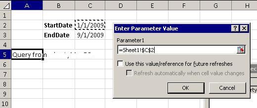
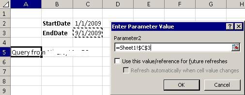
By applying ? (question-mark) in our query in WHERE clause Excel identifies them as 2 parameters and asks you from where to pick the data.

Now point both the parameters to the desired cell in the excel-sheet as shown below:

And finally you are done… when you will close the “Connection Properties” window the pivot report will get refreshed itself and pull the data as per the date you have applied.

Create an Excel Refreshable Report from database & Pivot Report

September 24, 2009 2 comments

Steps to create a Pivot Report

1. Open Excel Workbook, assuming that we are on sheet1.

2. Click on Data [Tab] — From Other Sources — From Microsoft Query

3. A new window will open “Choose Data Source”, and click OK button.

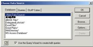
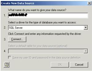
4. A new window will open “Create New Data Source”.
a. Provide the Data Source name, any name.
b. Select the Database Driver Name: SQL Server
c. Click Connect button.

5. A new window gets open “SQL Server Login”. Provide the DB credentials as shown above. Click OK button.

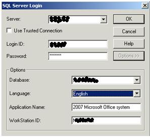
6. It will connect to the data-source.

7. Now Click on OK button of the “Create New Data Source” window as shown at step-4.
Leave the 4th step for the default table.

8. You will be prompted back to “Choose Data Source” window with a new Data Source entry you just created.

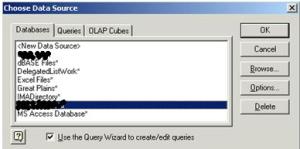
Select it and click on OK button.

9. A new window opens “Query Wizard – Choose Columns”.

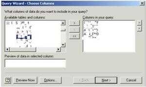
Select the number of columns you want to pull out and click on Next Button.

10. Click Next button repeatedly for the next 2 windows. In the final window “Query Wizard – Finish”…

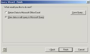
… select “View data or edit query in Microsoft Query” and click on Finish button.

11. You will be redirected to a new tool i.e. “Microsoft Query”.

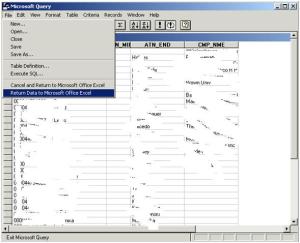
Here you can update your query, add new criteria and more filters.

When you are done with the query, go to the File menu and select “Return Data to Microsoft Office Excel”.

12. You will be redirected back to Excel with this new small window “Import Data”.

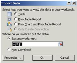
Choose your type of report & worksheet and then click on OK button.

13. You will get the data pulled out from the database for the specific query you applied, shown below:

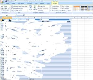
Click on the Refresh button to get the latest data.

14. To create a pivot report from this report on sheet1.

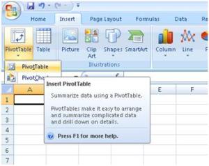
Click on sheet2 and click on Insert tab and select PivotTable from the drop-down menu as shown in window below.

15. A new window will appear “Create Pivot Table”.

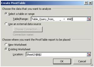
Select the source and destination table range as shown above. Click OK button.

16. PivotTable wizard is on the excel sheet and on the right side are the PivotTable field lists.

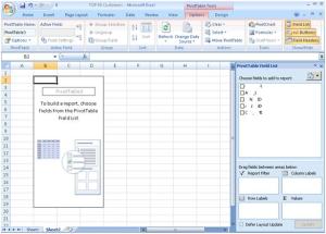
You can choose and drop the selected fields on the PivotTable area shown above.

Also you can apply filters and formulas to the PivotTable report.

17. The final PivotTable report is here.

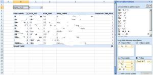
I’ve chosen 4 columns from the table (as shown inside the Row Labels box) and the 5th column is the derived column, count of Customers/Records (as shown inside the Value box).