SQL with Manoj

 
Steps to create a Pivot Report
 

1. Open Excel Workbook, assuming that we are on sheet1.

2. Click on Data [Tab] — From Other Sources — From Microsoft Query

3. A new window will open “Choose Data Source”, and click OK button.

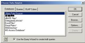
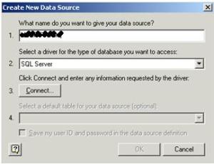
4. A new window will open “Create New Data Source”.
a. Provide the Data Source name, any name.
b. Select the Database Driver Name: SQL Server
c. Click Connect button.

5. A new window gets open “SQL Server Login”. Provide the DB credentials as shown above. Click OK button.

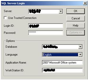
6. It will connect to the data-source.

7. Now Click on OK button of the “Create New Data Source” window as shown at step-4.
Leave the 4th step for the default table.

8. You will be prompted back to “Choose Data Source” window with a new Data Source entry you just created.

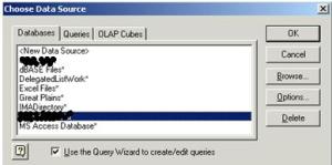
Select it and click on OK button.

9. A new window opens “Query Wizard – Choose Columns”.

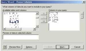
Select the number of columns you want to pull out and click on Next Button.

10. Click Next button repeatedly for the next 2 windows. In the final window “Query Wizard – Finish”…

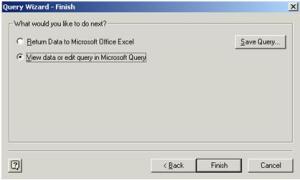
… select “View data or edit query in Microsoft Query” and click on Finish button.

11. You will be redirected to a new tool i.e. “Microsoft Query”.

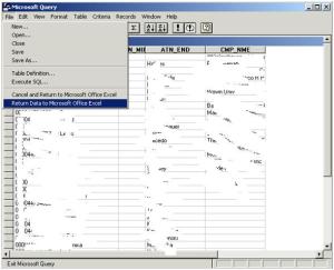
Here you can update your query, add new criteria and more filters.

When you are done with the query, go to the File menu and select “Return Data to Microsoft Office Excel”.

12. You will be redirected back to Excel with this new small window “Import Data”.

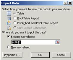
Choose your type of report & worksheet and then click on OK button.

13. You will get the data pulled out from the database for the specific query you applied, shown below:

Click on the Refresh button to get the latest data.

14. To create a pivot report from this report on sheet1.

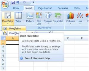
Click on sheet2 and click on Insert tab and select PivotTable from the drop-down menu as shown in window below.

15. A new window will appear “Create Pivot Table”.

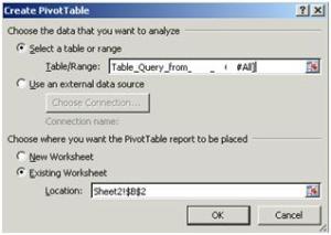
Select the source and destination table range as shown above. Click OK button.

16. PivotTable wizard is on the excel sheet and on the right side are the PivotTable field lists.

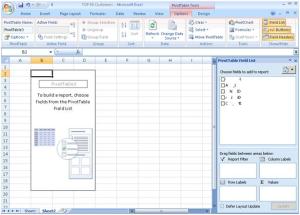
You can choose and drop the selected fields on the PivotTable area shown above.

Also you can apply filters and formulas to the PivotTable report.

17. The final PivotTable report is here.

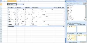
I’ve chosen 4 columns from the table (as shown inside the Row Labels box) and the 5th column is the derived column, count of Customers/Records (as shown inside the Value box).